Control Charts

Control charts are a way to monitor how a measurement behaves over time so you can quickly spot when a process or instrument drifts out of its expected range.

They are especially useful for running controls to confirm that a machine or instrument is still reading correctly (e.g., it should consistently read 1.0) and monitoring repetitive manufacturing processes (e.g., ensuring soda cans contain 20 ounces within acceptable limits).

Key Features

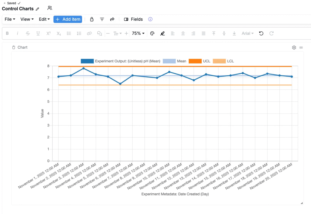
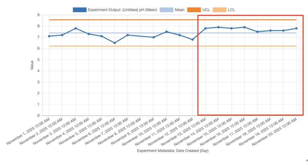
A typical control chart in Uncountable shows:

• Your measurements over time
• The mean value
• An Upper Control Limit (UCL), typically:
  • UCL = mean + (3 × standard deviation)
• A Lower Control Limit (LCL), typically:
  • LCL = mean − (3 × standard deviation)

When a point falls outside the control limits, it is a strong indication that something in your process, environment, or measurement system has changed and may need investigation.

Creating a Control Chart

Control charts are usually built on dashboard notebooks. To create a control chart on a dashboard:

Step 1 — Add a chart to your dashboard

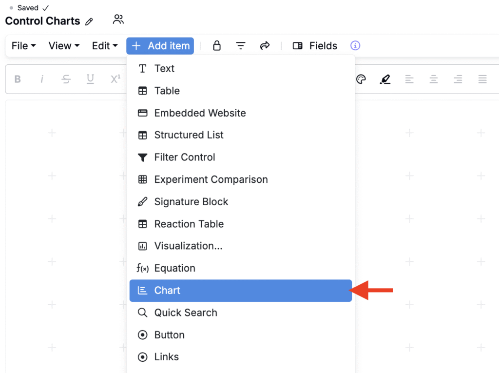
1. Open the relevant dashboard notebook.
2. Click Add item and select Chart.

Step 2 — Choose experiments and the parameter to plot

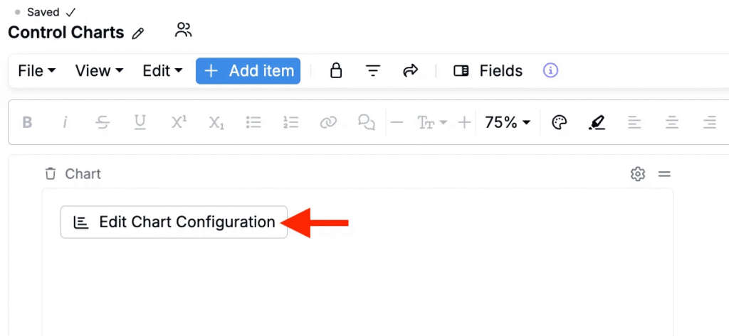
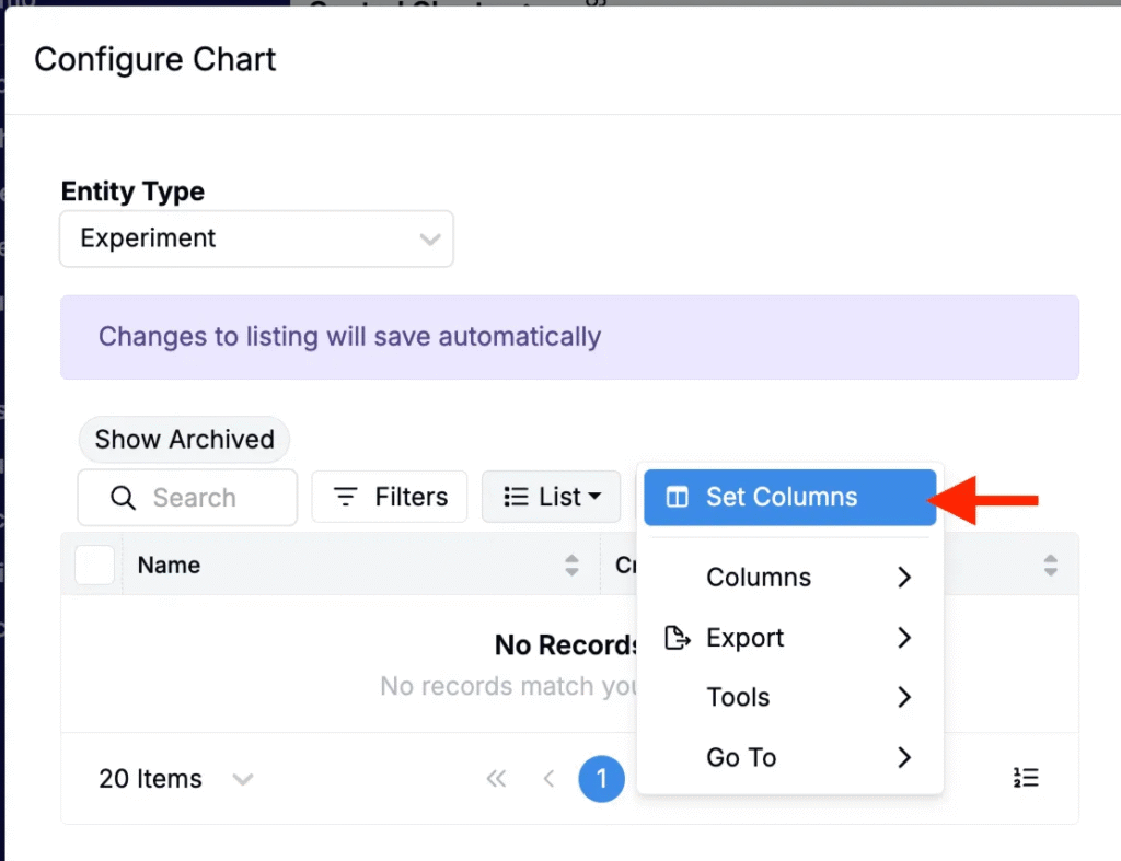
• Click Edit Chart Configuration.

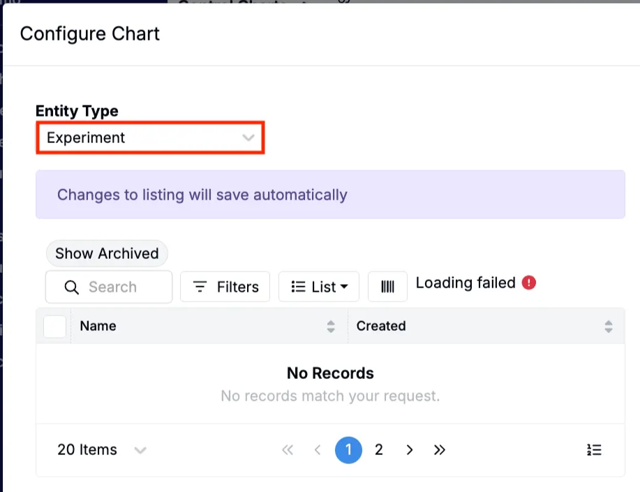
• Set Entity Type to Experiments.

• On the experiments listing, access the Select Columns modal (List > Set Columns).

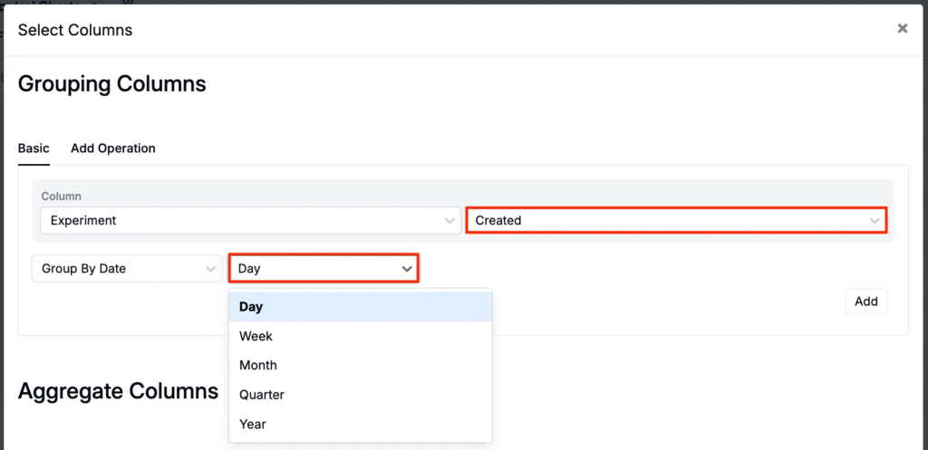
• In the modal, add an Experiments + Created grouping column.
  • You can choose to group by day, week, month, quarter, or year.

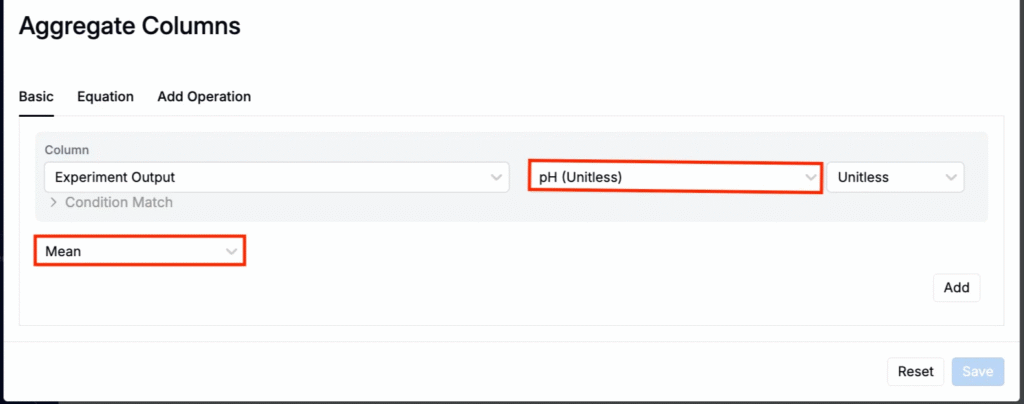
• Add a Experiment Outputs + [Output] aggregate column. Here, you can select any output you want to monitor (e.g., pH, Anode wet weight).
  • Set the aggregation to Mean (or another statistic, if appropriate). This ensures that if you record multiple measurements per day, they are averaged into a single value for that time bucket.

• Remove any extra identity columns you don’t need and save the configuration.
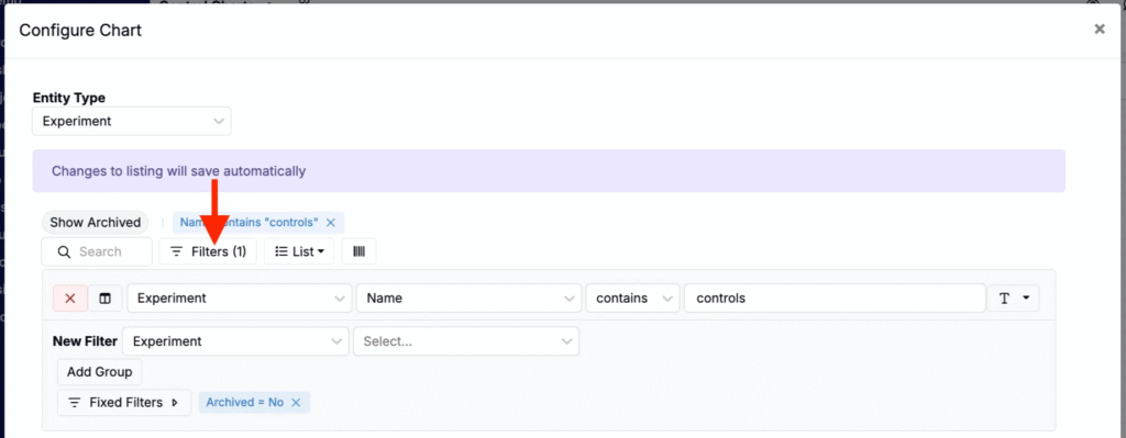
• Then add a filter to scope the listing table to include only the experiments that contain your control or process data.

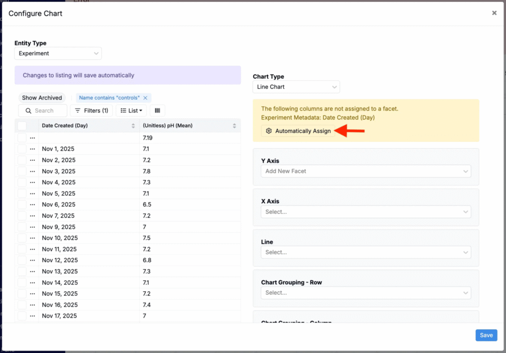
Step 3 — Assign axes

After configuring your fields:

1. Filter the listing table to include only the experiments that contain your control or process data.
2. Click Automatically Assign in the chart configuration.
3. Uncountable will typically:
   • Place your time field on the x-axis.
   • Place your mean measurement on the y-axis.

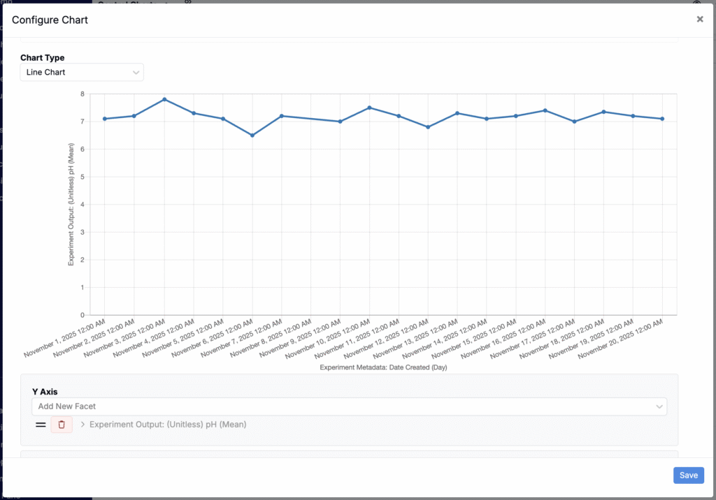
You can also manually assign axes, if needed.

At this stage, you have a basic trend chart: you can see how your control or process value changes over time.

Adding Control Limits

To turn your standard chart into a true control chart, you’ll add a line for mean, UCL, and LCL.

Step 4 — Create aggregates for mean, UCL, and LCL

In the chart configuration modal:

1. In the Aggregates section, add three aggregates on your experiment output.
2. For the Mean control limit:
   • Name: Mean
   • Equation: Mean
3. For the UCL (Upper Control Limit):
   • Name: UCL
   • Equation: Mean + 3 × stddev
4. For the LCL (Lower Control Limit):
   • Name: LCL
   • Equation: Mean − 3 × stddev
5. Save.

Note: The exact syntax depends on how aggregate equations are configured in your environment. Conceptually, you are always computing mean ± 3 × standard deviation for the same output you’re plotting.

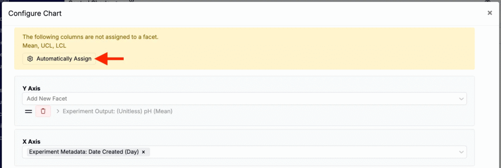
Step 5 — Add the aggregates as lines on the chart

After defining the aggregates:

• Click Automatically assign again, or manually assign the aggregates so they appear as reference lines across the chart.

• Optionally, adjust line color and styles by expanding the aggregate’s settings.

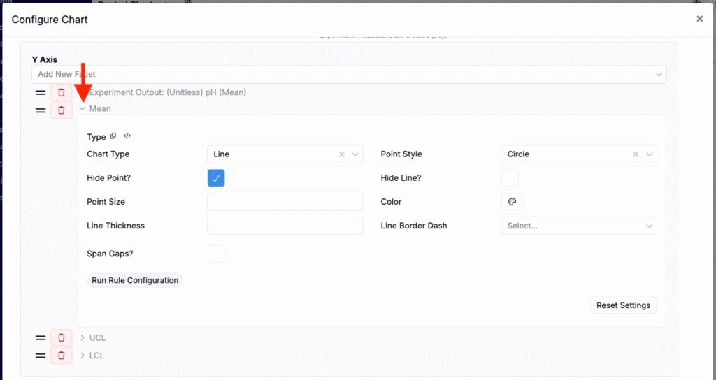
• Save the configuration.

Interpreting Control Charts

Because the chart is on a dashboard notebook, it updates automatically when you record new measurements for the same parameter. If you are running regular controls (e.g., daily instrument checks), the control chart becomes a live view of your current process health.

Some common patterns to watch for:

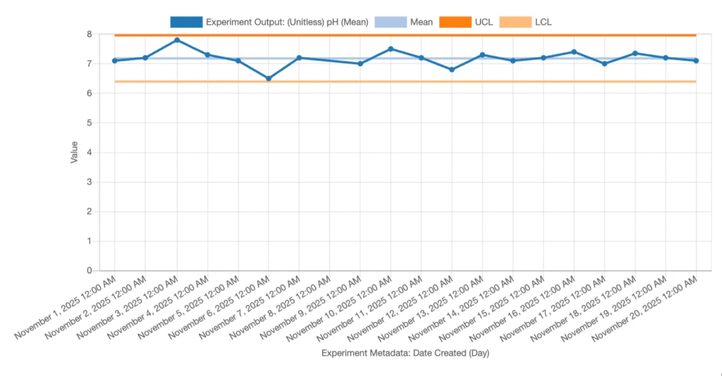
• Points inside UCL/LCL with no strong pattern
  • Process is likely stable and behaving as expected.

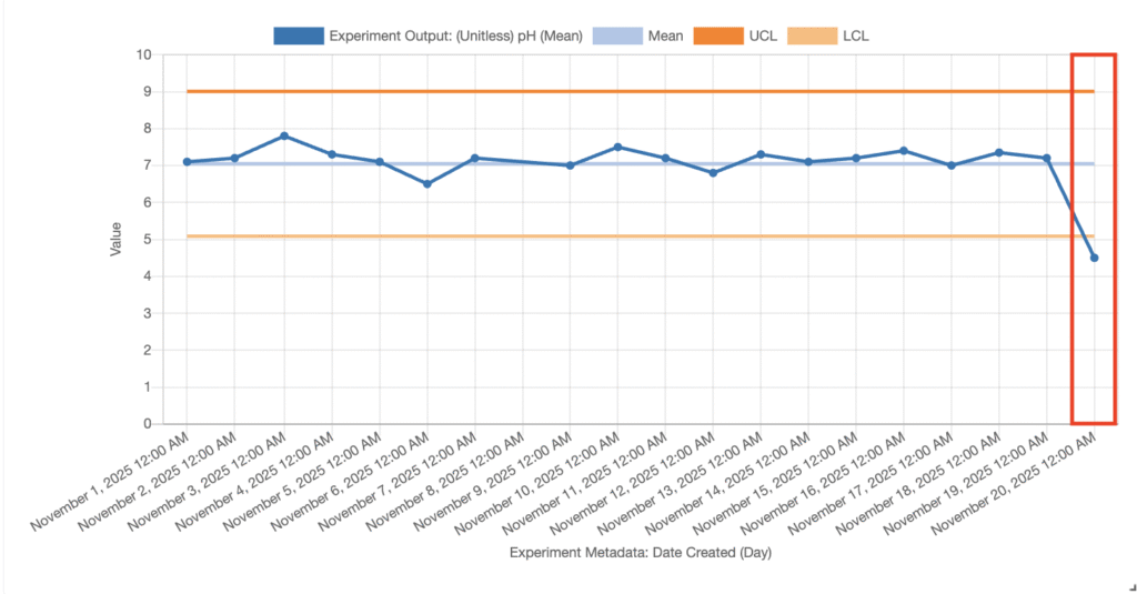
• Point above UCL or below LCL
  • Strong signal that something in your process or measurement system has changed.
  • Investigate machine calibration, materials, method changes, or data entry issues.

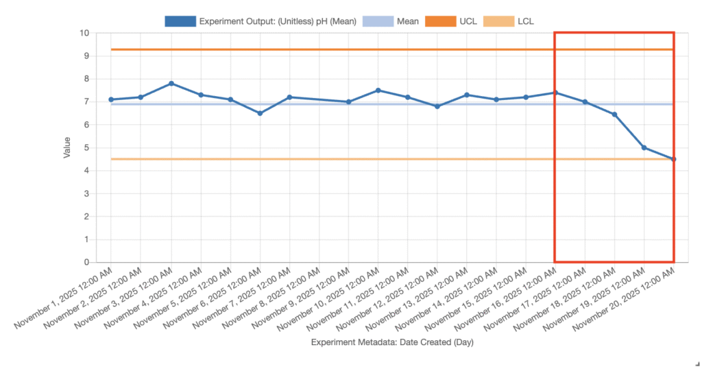
• Trend over time (e.g., gradual drift upward)
  • May indicate progressive drift in equipment or a slow change in process conditions.

• Sequence of points on one side of the mean
  • Can indicate a shift in the mean, even if points are still within UCL/LCL.

Use these signals to check or recalibrate instruments, review recent process changes, or decide whether to pause production or adjust process settings.

Key Takeaways

• Control charts track a measurement over time and surface drift using the mean plus upper and lower control limits (typically mean ± 3σ).
• Build them in dashboard notebooks by charting your output, grouping by time, averaging within each time bucket, and filtering to the relevant experiments.
• Add aggregates for Mean, UCL, and LCL, then assign them as reference lines so limits are visible on the chart.
• Interpret signals: points outside limits, persistent trends, or long runs on one side of the mean suggest investigation or recalibration. </aside>