
Curve Similarity Search extends Objective Search to compare curve-shaped outputs and find experiments with similar profiles. Instead of ranking recipes by how close they are to numeric goals, this mode evaluates shape similarity between curves and returns the most comparable results.
When to Use Curve Similarity
Use Curve Similarity when you need to:
- Identify experiments with similar signal or shape patterns, even if their absolute values differ.
- Compare spectroscopic, mechanical, or thermal data to a known performance curve.
- Find reference or baseline matches for further analysis.
Common use cases include IR and UV–Vis spectra, DMA curves, and DSC thermograms.
Accessing Curve Similarity Search
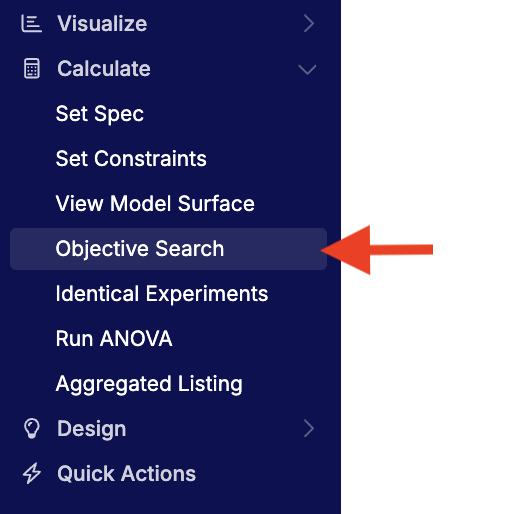
Open Objective Search from the Calculate tab.
Running a Curve Similarity Search
- Under Goals, confirm the spec output you’re searching on is a curve-type output. Only curve outputs are supported in this mode.
- Use the Target Curve dropdown to choose the reference curve you want to match. This could be a known material behavior, a previous benchmark, or a desired response profile.

Understanding the Results
After running the search, the Top Results table ranks recipes by how well they meet your spec.
- Columns show recipes, sorted by Rank (best matches on the left)
- Rows list curve similarity
- 0% means no similarity between the two curves
- 100% means the two curves are (almost) identical

How Similarity Is Calculated
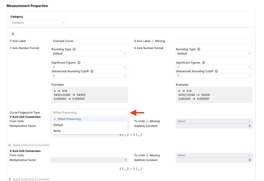
Curve Similarity Search offers two fingerprint types, each with a different approach to comparing curves. The fingerprint type for a curve calculation can be set on that curve’s output’s Details page.
Default (Shape-Based)
The Default fingerprint type normalizes the X and Y axes and compares curves based on shape alone:
- Normalization — The x-axis is scaled to
[0, 1]and the y-axis is centered to a mean of 0. - Fourier Transform — A nonequispaced discrete Fourier transform (n = 100) captures frequency-domain features of the curve.
- Cosine Similarity — The transformed curves are compared using cosine similarity to produce a similarity score between 0–100%.
This method emphasizes shape similarity rather than peak position or amplitude. Minor shifts in the x-axis (e.g., slightly offset peaks) can still produce high similarity scores.
For example, if you had a set of curves like this:
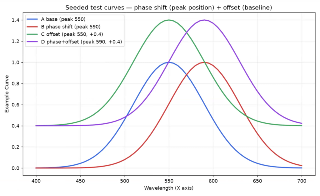
You would generate a similarity score like these:

These scores are similar, since the curves were close in shape, despite their offsets.
Offset Preserving (Position-Aware)
The offset-preserving fingerprint type retains X/Y offset information instead of normalizing it away, and uses L2 norm (Euclidean distance) instead of cosine similarity to compare curves. This means differences in both shape and absolute position are reflected in the score.
This method is recommended when absolute curve position matters — for example, when matching spectral curves where a peak at 450 nm (blue) and a peak at 650 nm (red) should not be considered similar.
To switch fingerprint types, use the Fingerprint Type dropdown in the Objective Search panel and choose Offset Preserving.
In this case, if you had the same set of curves shown above, you would get a lower similarity score:

This is because, despite the fact that the curves are similar in shape, their positions are offset.
Tips and Notes
- Permissions still apply: if you can’t view outputs or recipes, those results won’t appear.
- If curves with different X/Y offsets are scoring too similarly with the default fingerprint type, try switching to Offset Preserving to retain offset information.
- If the Spec Type dropdown doesn’t include Curve Similarity, verify that the chosen output is a curve-type output.
- The Target Curve must have valid recorded data for the selected output.
- Filters applied in Objective Search also apply here — overly restrictive filters can limit your result set.