Analyze with AI

Uncountable ML Overview

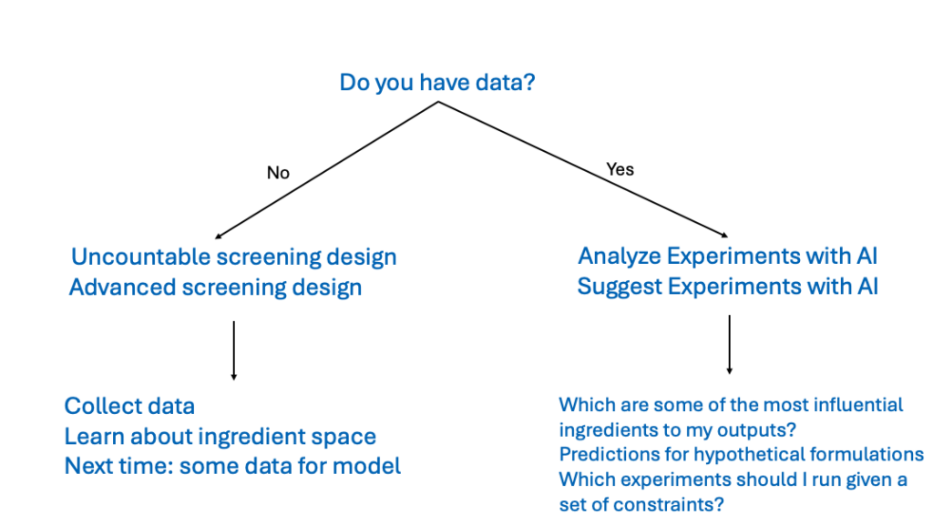
The Uncountable platform includes AI tools designed to analyze past data, generate predictions, and suggest future experiments.

To use these tools, users must have existing experimental data for the platform to create accurate predictive models. If no data is available yet, use Advanced Screening Design (DOE) to generate datasets first.

Once sufficient data has been collected, the Analyze with AI and Suggest with AI tools can help identify which inputs have the strongest influence on outputs, predict outcomes for hypothetical formulations, and guide future experimentation with actionable suggestions.

Analyze with AI

Analyze with AI is an Uncountable ML design tool that builds predictive models from your existing experimental data. With a trained model, you can estimate how a formulation or experiment will perform in specific tests before running new lab work, or in some cases, without running the test at all.

Analyze also helps you evaluate how reliable your dataset is for prediction. If key measurements are noisy or don’t vary much, the model’s predictive strength may be limited.

If a formula or experiment includes inputs that aren’t in the model, the platform will suggest the closest available substitute. If no substitute is appropriate, or if the missing input is important, add it to your model constraints and retrain the model.

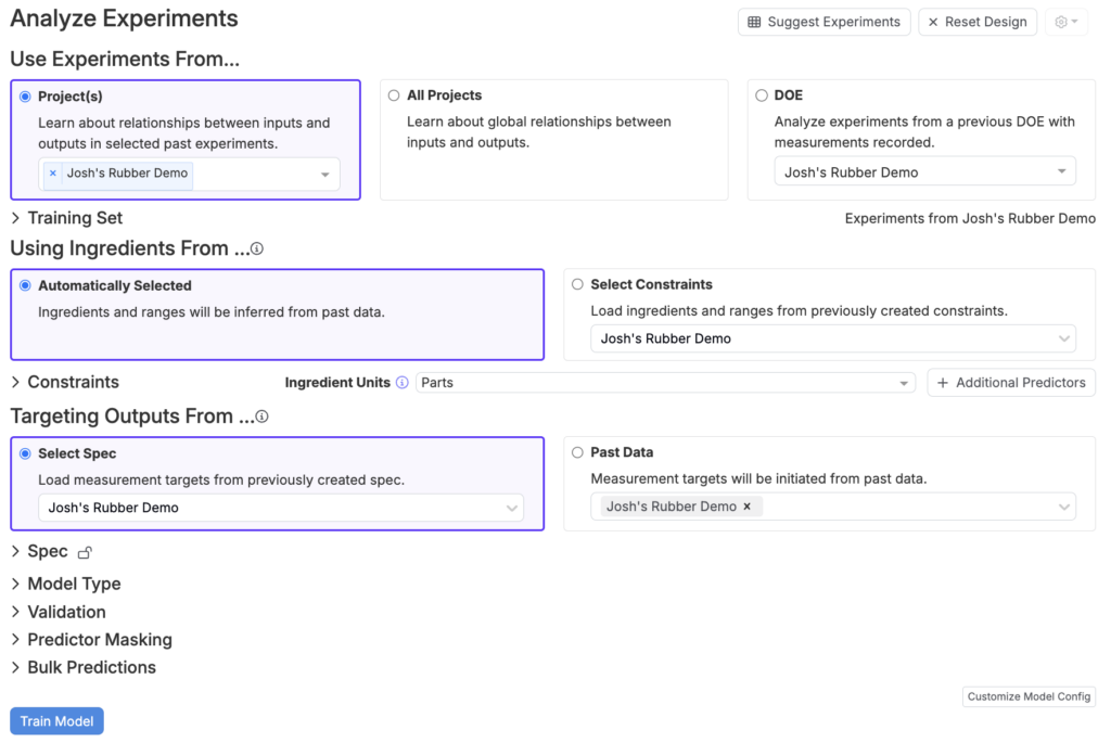
Uncountable’s Analyze with AI design tool

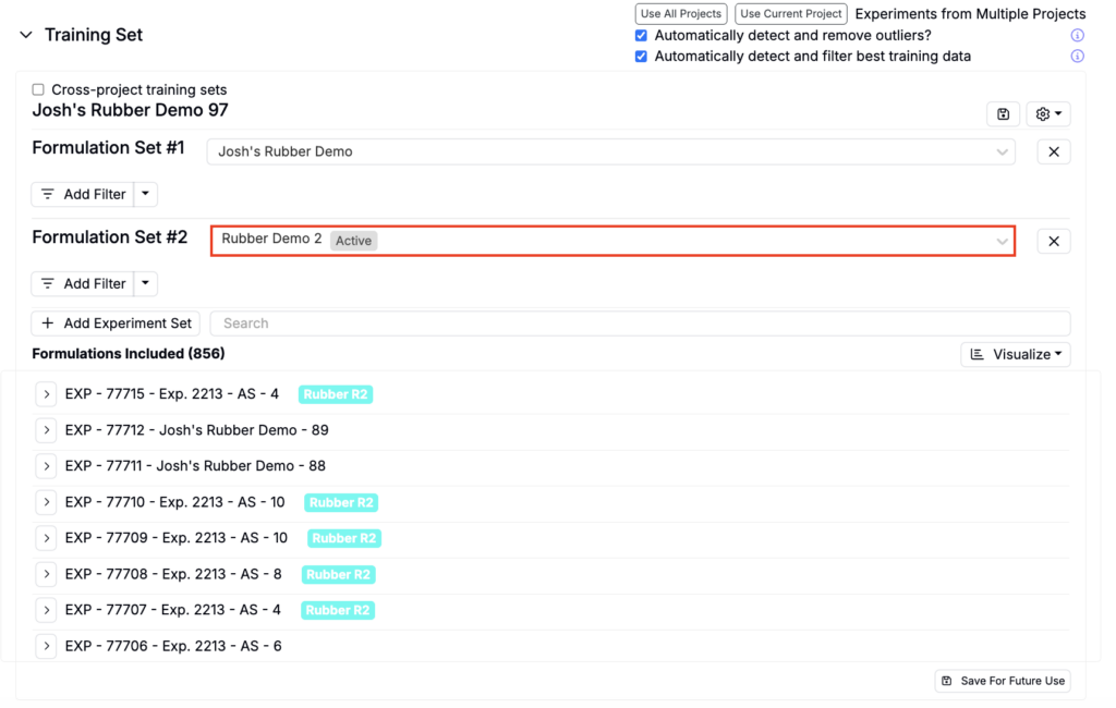
Step 1 — Creating a Training Set

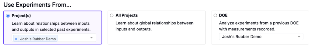
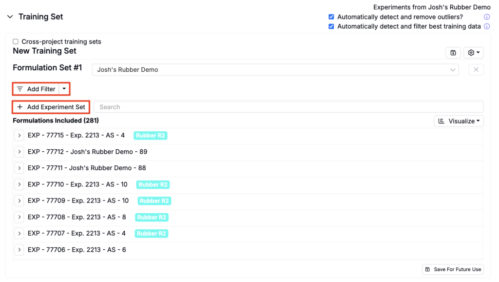
To run an Analyze job, begin by selecting experiments from one of the following:

• Project(s) — Use only the recipes and results from a selected project or projects. This is the recommended option for most scenarios, as it ensures a consistent set of ingredients, process parameters, and measurements relevant to the current project.
• All Projects — Include data from all projects within the current material family. This option broadens the training set, which can improve model generalization by incorporating diverse historical data. However, use this option only if you are familiar with and have access to data outside the current project.
• DOE — Focus solely on experiments from a DOE previously created in Uncountable. Note that DOE data is automatically included when selecting the Project(s) option.

Under Training Sets, refine experiments by adding filters, and/or additional formulation sets.

Excluding Experiments/Measurements

In addition to adding filters, you may want to include or exclude additional experiments.Consider excluding experiments if:

• They are significant outliers in terms of ingredient types or amounts
• Input data, especially for important parameters, is missing or incomplete
• Data from the experiment is unreliable

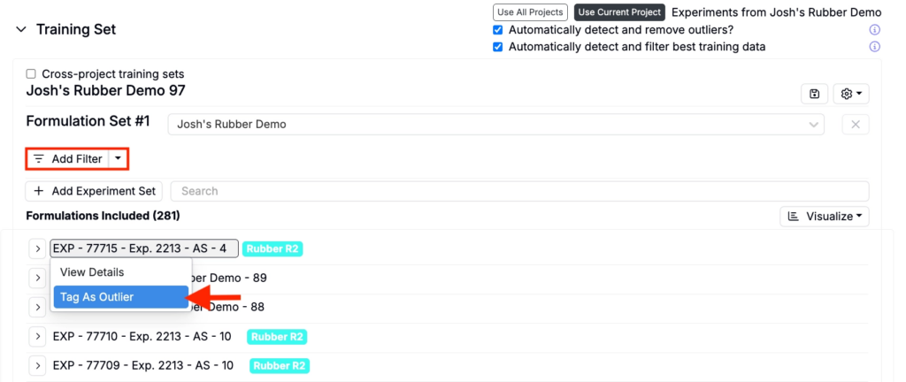
To exclude an experiment add filters or manually mark experiments as outliers by clicking the experiment name and selecting Tag as Outlier.

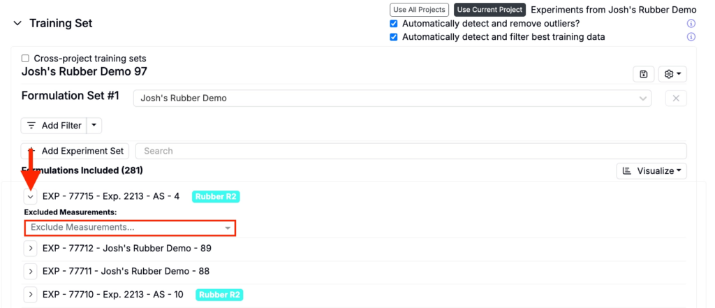
To exclude specific measurements from an experiment, expand the experiment and use Excluded Measurements to select the measurements you want to exclude.

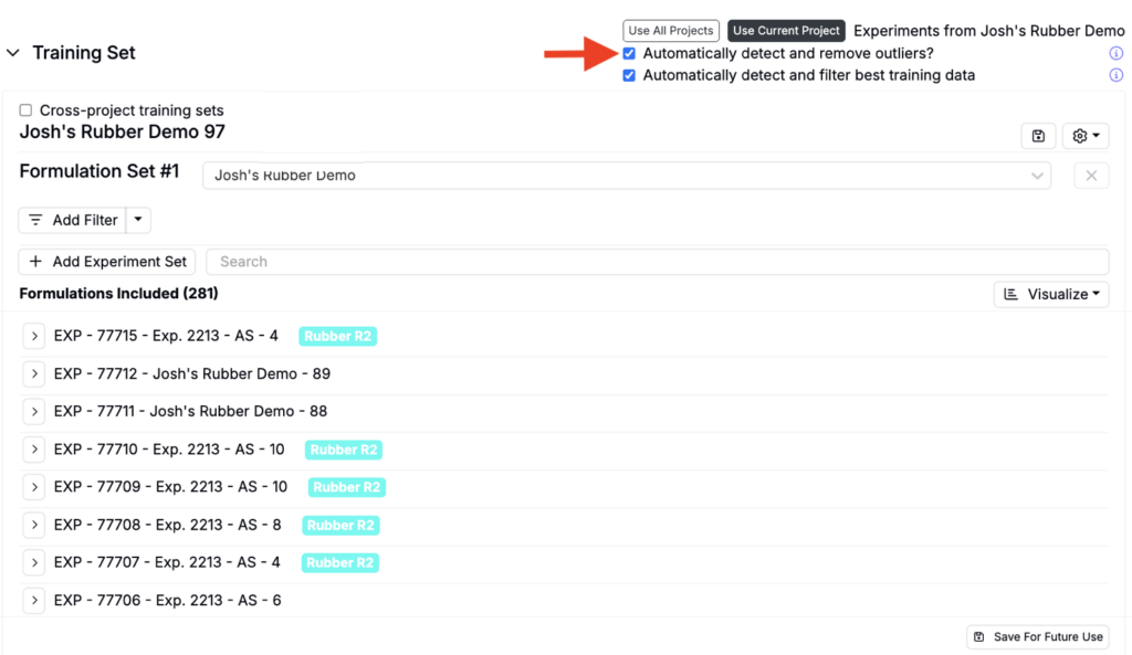
Excluding Outliers

By default, Suggest will automatically detect and remove outliers to exclude data points that fall outside statistical thresholds. To include outliers, uncheck the Automatically detect and remove outliers setting at the top of the Training Set section.

Including Experiments

Experiments should be included when:

• They don’t meet any of the exclusion criteria above, or
• If they belong to a different project but are closely related to your current data set.

To include additional experiments, click the Add Experiment Set button, select a project, and add additional filters.

For more information on how much data is needed to build effective prediction models, refer to this article.

Step 2 — Selecting Input Features

Next, select the input features from the training set that the model will use to make predictions. Input features, such as ingredients, process parameters, and calculations are the independent variables your model relies on to predict outputs.

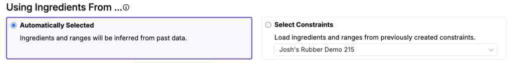
There are two options when selecting input features:

• Automatically Selected — By default, the Uncountable platform automatically selects the most common input features in your dataset.
• Select Constraints — Alternatively, users can manually define constraints for input features to customize model training.

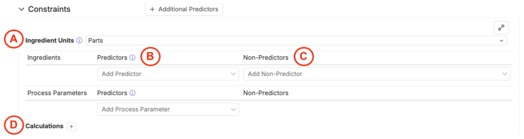
To manually configure constraints, expand the Constraints section. This allows users to define:

• Ingredient Units (A): Specify the unit type for sampled experiments.
  • Percentage Units: Experiments with percentage units will always sum to 100%.
  • Parts Units: Experiments with parts units may sum to arbitrary values, depending on the setup.
• Predictors (B): Ingredients and process parameters marked as predictors are used to calculate output performance and experiment properties (i.e. cost or density). Predictors directly influence the model’s ability to make accurate predictions.
• Non-Predictors (C): Ingredients and process parameters designated as non-predictors can still be used to calculate experiment properties but do not directly affect output performance predictions.
• Calculations (D): Define input calculations, such as “Cost per Experiment,” to either set constraints for suggestions (for example, keep cost below a threshold or within a range) or run what‑if analyses during Analyze (for example, reduce cost by 5%) to see how the change affects the outputs you selected.

For additional guidance on setting up effective constraints, refer to this article.

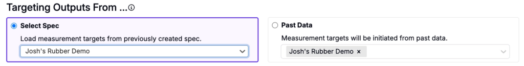
Step 3 — Targeting Outputs

Next, select the measurements of interest (what the model will predict). There are two options when selecting outputs are:

• Select Spec — Use a previously created spec associated with the current project or any project selected from the dropdown menu. The spec will be used to identify measurements of interest.
• Past Data — Use past data from a selected project to identify measurement targets.

Under Spec, users can view the target measurements and adjust type, priority, and settings.

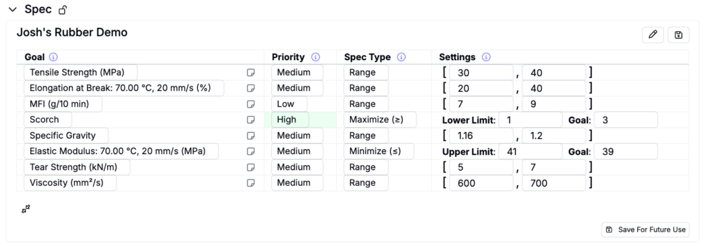
When building a model for analysis only, rather than generating recommended experiments, you do not need to set priorities or thresholds for the spec. The platform automatically creates a separate model for each selected measurement of interest, and these priorities or goals do not influence how the model is built.

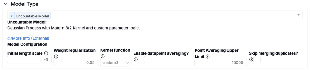
Step 4 — Selecting a Model Type

Uncountable Model (Matérn-kernel Gaussian Process)

The Uncountable platform is powered by Uncountable’s proprietary models, which are built on a Matérn-kernel Gaussian Process (GP). This GP model underpins much of the platform’s functionality and is the default model type for Analyze jobs.

Other Models

For comparative analytics, users can also train and analyze a variety of alternative models alongside the Uncountable GP model. These models, which are also suitable for predictive purposes, can be visualized using surface visualizations. The available models include:

• Linear Regression
• Ridge Regression
• Random Forest
• Neural Network
• Decision Tree Regression
• SVM
• Gradient Boosting Regression (via XGBoost)
• K Neighbors Regression

If multiple models are trained, the platform provides a separate training accuracy table for each, enabling direct comparison to determine which model best fits your data.

Tuning a Model

Each model offers specific hyperparameters for tuning. For instance:

• Gaussian Process (GP): Adjust initial length scale, weight regularization, or kernel function types.
• Random Forest: Configure the number of estimators, maximum tree depth, and the criterion function.

For more details on Uncountable’s modeling approach, visit this article.

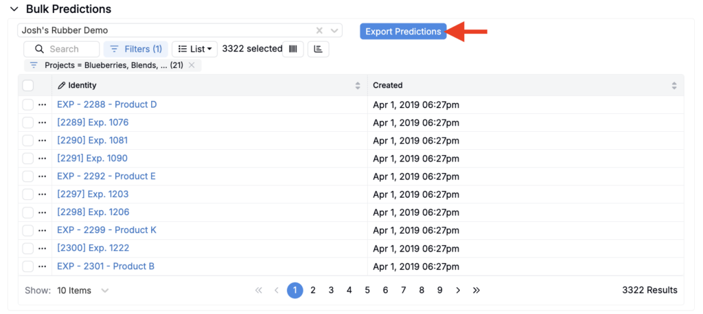
Bulk Predictions (Optional)

The standard Analyze with AI feature limits how many experiments you can include in a single prediction run. For larger batches (up to 20,000 experiments at once), use Bulk Predictions.

To generate bulk predictions:

1. Select the model you want to use.
2. Use filters to define which experiments to include.
3. Click Export Predictions to start the asynchronous export.

After the export is complete, you will receive an output that includes variables, variable types, predicted values, and any associated errors for all selected experiments.

Step 6 — Training/Interpreting the Model

Once model settings have been configured, click the Train Model button to run the initial training job.

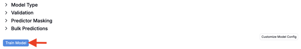
Once the job is complete, results will be displayed below. If adjustments are needed after reviewing these sections, users can reconfigure input or output settings and rerun the model to refine predictions and analysis.

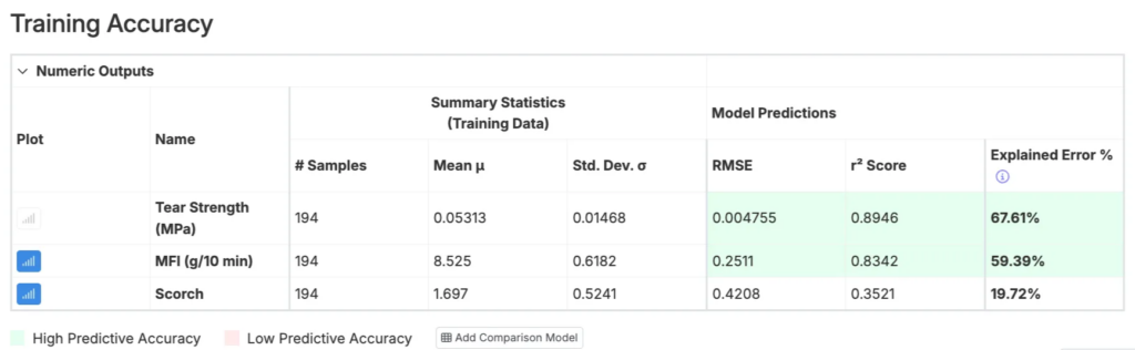
Training Accuracy Table

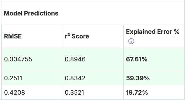
The Training Accuracy table informs the user about the performance of the model, displaying summary statistics and model predictions for each output.

• RMSE: Measures the predictive error of the model, with lower values indicating greater accuracy.
• r² Score: Reflects the explanatory power of the model, with values closer to 1 indicating better performance. It measures how much of the variance in the output data is accounted for by the model.
• Explained Error: Normalizes RMSE relative to the standard deviation of the dataset. This comparison accounts for differences in magnitude across outputs, enabling consistent evaluation. Higher values, closer to 100%, signify more accurate model predictions.

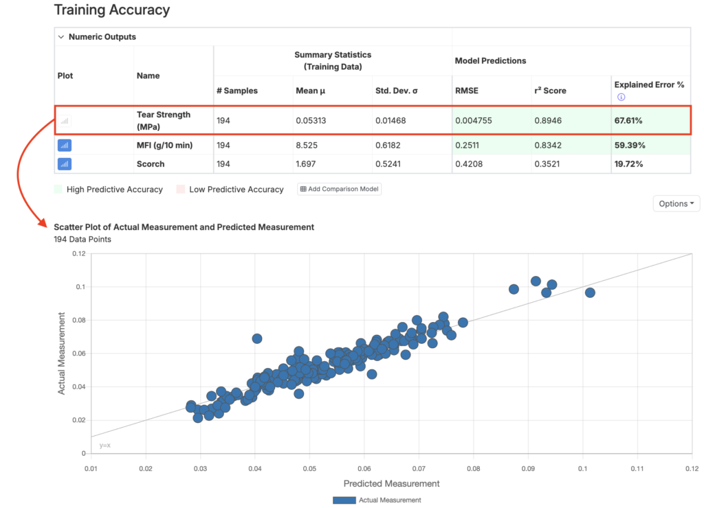
Training Accuracy Scatter Plot

The Training Accuracy scatter plot provides a visual representation of the predictive quality of a selected output (i.e. Tear Strength) by comparing predicted values against actual measurements. To select an output for the plot, click the corresponding plot icon in the Training Accuracy table.

The scatter plot is an intuitive and informative way to evaluate model predictions. The Uncountable platform uses all current data points to predict one another, plotting these predictions against their actual values. Ideally, points should align near the diagonal gray line, which represents y = x (perfect predictions), though some deviation is expected in practice.

Interpreting the Scatter Plot

When interpreting the training accuracy scatter plot, pay attention to the following:

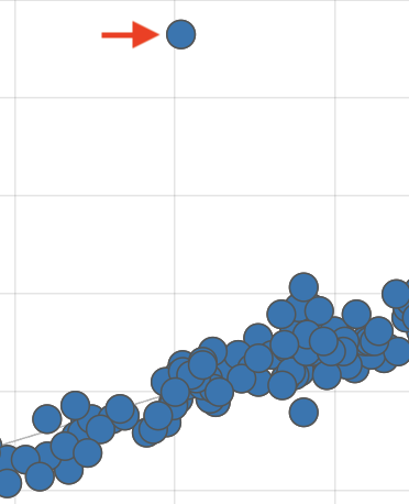
• Outliers: Look for data points significantly deviating from the diagonal line. These could indicate unreliable measurements. To address this:
  • Remove unreliable data points from the training dataset.
  • Tag them as outliers on the Dashboard or Enter Measurement page.

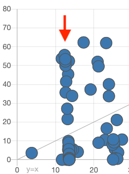
• Vertical Lines: If multiple points form vertical lines on the plot, it suggests that the model is producing the same prediction for different actual measurements. This could be caused by:
  • Missing Input Features: Ensure all critical ingredients and process parameters are included in the constraints used to create the model.
  • Incomplete Process Parameter Data: Blank fields are interpreted as “0” by the model. Remove incomplete data points or exclude these parameters from the model features.
  • Hidden Subgroups in the Data: Verify that the experiments in the dataset are not from distinct groups or conditions that should not be mixed together.

Effect Sizes

The Effect Sizes Table illustrates how each input in the model influences a specific output, providing a clear view of the relationship between ingredients or parameters and the resulting measurements.

• Each value represents the effect size of an input on the output, displayed as a percentage of the output’s standard deviation. Positive effects are marked in blue, while negative effects are shown in red, making it easy to identify the direction of influence.
• A positive effect size indicates that an increase in the input increases the output, while a negative size means that an increase in the input decreases the output.
• Clicking on an output’s column header allows users to sort inputs by their impact on the chosen output.
• Larger effect sizes (i.e. above 150%) may signal strong trends or potential anomalies in the data. It’s important to confirm whether these trends align with scientific expectations or if adjustments to the model or data are needed.
• For projects with cumulative ingredient effects or limited individual input impact, weaker trends in the table are common. In these cases, understanding the balance of all ingredients becomes more critical.
• Cross-referencing the Effect Sizes Table with tools like View Correlations or Explore Data can help validate the model’s findings and ensure accurate interpretation.

Model Plots

In the Model Plots section, users can use surface and scatter plots to explore how two input parameters affect a single output.

• Select inputs for the X and Y axes
• Select an output for the color
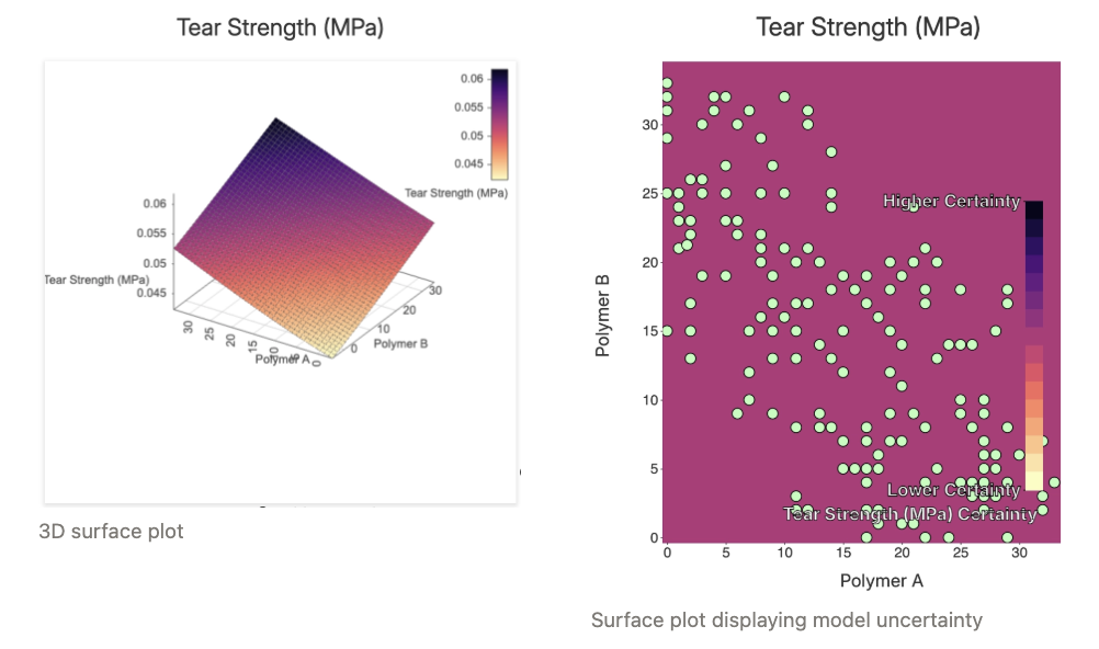
• Use the settings in the top right to display model uncertainty or to switch to a 3D plot

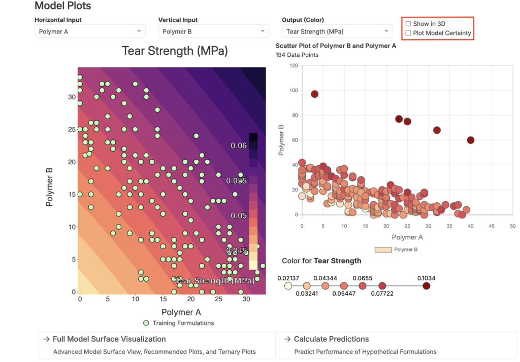
Model plots are useful for examining the interactions between two ingredients, revealing how they might work together synergistically or represent trade-offs. However, it’s important to compare these model-generated plots with scatter plots or bar charts derived directly from the data to ensure the model’s predictions align with real-world observations.

Interaction Explorer

While model plots are limited to showing two inputs and one output at a time, the Interaction Explorer allows for more complex visualizations involving multiple inputs.

Using the Interaction Explorer, users can select several inputs and an output to see how the predicted output changes based on different combinations of input values. By manually adjusting the vertical blue line for each input, the plot will dynamically update, showing how the predictions change as the input values are altered.

Understanding Predictions

The main purpose of creating a model is to make accurate predictions about formulations or experiment outcomes without the need to perform lab tests. Once your model is built and demonstrates good predictive accuracy, it can help you estimate results based on previous data.

If a formula or experiment has missing inputs that aren’t part of the model, the platform will suggest the closest substitute. If no suitable substitute is available, or if the missing input is crucial, you can add it to your model’s constraints and retrain the model.

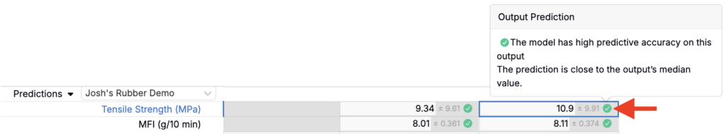
Predictions are shown with three confidence levels:

• Green: High confidence with low error.
• Yellow: Moderate confidence.
• Red: Low confidence, and the prediction should not be trusted.

Low confidence could be due to inputs falling outside the data’s range, low accuracy for the measurement, or insufficient data. In rare cases, predictions may yield unrealistic values, such as negative numbers for measurements that should be non-negative. This happens because the model does not account for physical limitations and predicts across the entire range. If this occurs, treat negative values as predictions of zero.

Saving/Loading a Model

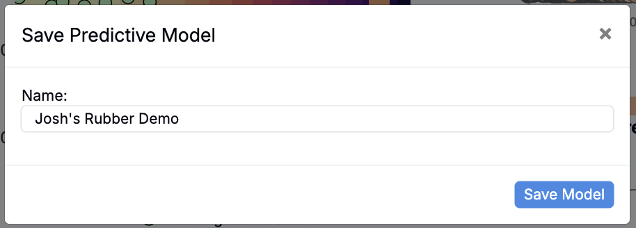
Once a predictive model is complete, it can be saved for future use by clicking the Save Model button at the bottom of the page. While all models are saved automatically by default, clicking this button lets you give the model a custom name for easier identification and access.

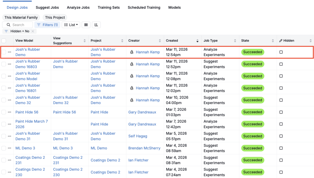
To access a saved or previously run model, navigate to the View Past Jobs page by selecting Design > View Past Jobs. Here, you’ll find a listing of all previously run models. Models cannot be deleted, but they can be “Hidden”.

Exposing Predictions

Once you have predictions for an experiment, a common next step is to expose them during data entry. Predictions are most useful for relative ordering (which recipe is expected to perform better) rather than as exact point values.

To expose model predictions on the Recipe view of experiments:

• Save the model (predictions can only be shown for saved models).
• From the your project Dashboard, select the recipes/experiments you want to view predictions for and open the Recipe view of these experiments.
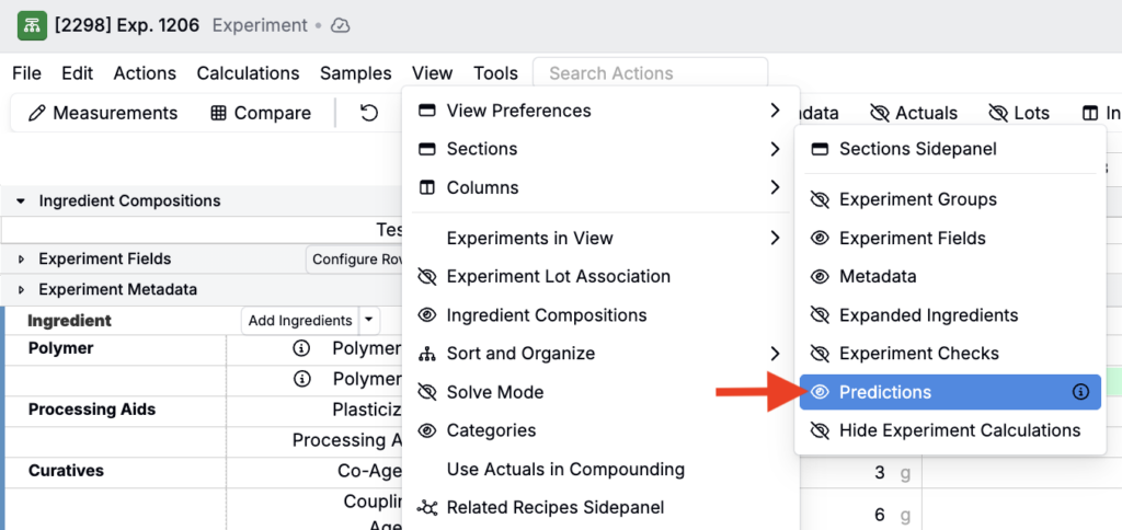
• In the View menu, select Sections > Predictions to enable the Predictions section.

• At the bottom of the page, select the saved model and click Get Predictions.

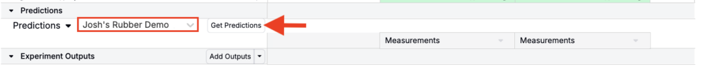
Output predictions for each experiment will appear within the Predictions section. Click into each output cell to view more information.